The objective of this experiment is to design a DC Motor position controller using Root Locus Method considering disturbance in the system and reduce the effect of the disturbance to zero.
Root Locus:
The root locus of an open loop transfer function H(s) is a plot of the locations (locus) of all possible closed loop poles with proportional gain k and unity feedback:


And thus the poles of the closed loop system are values such that 1 + KH(s) = 0
No matter what the pick k to be, the closed loop system must always have n poles, where n is the number of poles of H(s). The root locus must have n branches; each branch starts at a pole of H(s) and goes to a zero of H(s). If H(s) has more poles than zeros, m
Characteristics:
Since the root locus is actually the locations of all possible closed loop poles, from the root locus can be selected such a gain that the closed loop system will perform the way it is required.
ü If any of the selected poles are on the right half plane, the closed loop system will be unstable.
ü The poles that are closest to the imaginary axis have the greatest influence on the closed loop response, se even though the system has three or four poles, it may still act like a second or even first order system depending on the locations of the dominant poles.
Design requirements:
If simulation was done with the reference input r(t) by a unit step input, then the motor speed output should have
ü Settling time less than 40 milliseconds
ü Overshoot less than 16%
ü No steady state error
ü No steady state error due to a disturbance
Mathematical analysis:
The motor torque T is related to the armature current, I by a constant factor Kt. The back emf, e, is related to the rotational velocity by the following equations.
T = KIi
e = Keθ
From the figure, we can write the following equations.

Where,
J=moment of inertia of the rotor
b=damping ratio of the mechanical system
K=Kt=Ke=electromotive force constant
R=electric resistance
L=electric inductance
V=source voltage
θ=position of shaft
Using

In order to meet the design specification, a feedback system with an appropriate controller is developed which is shown below and has a transfer function of

Where,
Kp = Proportional gain
KI = Integral gain
KD = Derivative gain
Motor Parameters:
1. Moment of inertia of the rotor (J) = 3.2284x10- 6 kg-m2/s2
2. Damping ratio of the mechanical system (b) = 3.5077x10- 6 Nms
3. Electromotive force constant (K = Ke = Kt) = 0.0274 Nm/Amp
4. Electric resistance (R) = 4 Ω
5. Electric inductance (L) = 2.75x10- 6 H
6. Input (V) = Source Voltage
7. Output (θ) = position of shaft
8. The rotor and shaft are assumed to be rigid
MATLab Code:
clear;
clc;
clf;
close all;
% Open Loop System
J = 3.2284e-6;
b = 3.5077e-6;
K = 0.0274;
R = 4;
L = 2.75e-6;
num = K;
den = [(J*L) ((J*R)+(L*b)) ((b*R)+K^2) 0];
sys = tf(num,den);
subplot(311), step(sys,0:0.001:0.2);
grid on;
title('Step Response for Open Loop System');
xlabel('Time (seconds)');
ylabel('Position (rad)');
% Proportional Control
kp = 1.7;
closed_sys = feedback(sys*kp,1);
subplot(312), step(closed_sys,0:0.001:0.2);
grid on;
title('Step Response for Kp = 1.7');
xlabel('Time (seconds)');
ylabel('Position (rad)');
% Disturbance Response
dist_sys = closed_sys/kp;
subplot(313), step(dist_sys,0:0.001:0.2);
grid on;
title('Step Response for Disturbance for Kp = 1.7');
xlabel('Time (seconds)');
ylabel('Position (rad)');
% Drawing the Root Locus
figure;
subplot(211), rlocus(sys);
sgrid(0.5,0);
axis([-400 100 -200 200]);
title('Root Locus - P Controller');
% Integral Control
numcf = [1];
dencf = [1 0];
controller = tf(numcf,dencf);
I_sys = controller*sys;
subplot(212), rlocus(I_sys);
sgrid(0.5,0);
axis([-400 100 -200 200]);
title('Root Locus - I Controller');
% Proportional plus Integral Control
numcf = [1 20];
dencf = [1 0];
controller = tf(numcf,dencf);
PI_sys = controller*sys;
figure;
subplot(211), rlocus(PI_sys, 0:0.1:30);
sgrid(0.5,0);
axis([-400 100 -200 200]);
title('Root Locus - PI Controller');
% Proportional plus Integral plus Derivative Control
numcf = conv([1 60],[1 70]);
dencf = [1 0];
controller = tf(numcf, dencf);
PID_sys = controller*sys;
subplot(212), rlocus(PID_sys, 0:0.001:1);
sgrid(0.5,0);
axis([-400 100 -200 200]);
title('Root Locus - PID Controller');
% Finding the gain using the rlocfind command
figure;
rlocus(PID_sys,0:0.001:1);
sgrid(0.5,0);
axis([-400 100 -200 200]);
title('Root Locus - PID Controller');
% Step Response for Compensated System
[k poles] = rlocfind(PID_sys);
feedbk_sys = feedback(k*PID_sys,1);
figure;
subplot(211), step(feedbk_sys, 0:0.001:0.1);
grid on;
title('Step Response for Compensated System');
ylabel('Position (rad)');
% Step Response for Compensated System for Disturbance
dist_sys = feedbk_sys/(k*controller);
subplot(212), step(dist_sys, 0:0.001:0.1);
grid on;
title('Step Response for Compensated System for Disturbance');
ylabel('Position (rad)');
MATLab Simulation:

Figure: Step response for Open Loop System and Proportional Controlled Closed System

Figure: Root Locus for Proportional and Integral Controlled Closed

Figure: Root Locus for PD and PID Controlled Closed System
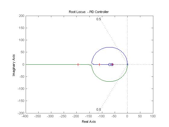
Figure: Root Locus for Proportional Derivative Integral Controlled Closed System

Figure: Step response for Compensated System
In this experiment a PID controller was designed with root locus method, to fulfill the requirements given.
No matter what is the value of K in the control system above, the closed loop system must always have n poles, where n is the number of poles of H(s). The root locus must have n branches; each branch starts from a pole and goes to a zero of H(s). If H(s) has more poles than zeros M < n and we say that H(s) has zeros at infinity. In this case, the limit of H(s) as s ≥ µ is zero. The number of zeros at infinity is n – M, the number of poles minus the number of zeros, and is the number of branches of the root locus that go to infinity (asymptotes).
Root locus method:
The relative stability and the transient performance of a closed loop control system are directly related to the location of the closed-loop roots of the characteristic equation in the s-plane. It is useful to determine the locus of roots in the s-plane s a parameter is varied. Thus by determining the locus of the roots in the s-plane as a parameter is varied it is possible to meet the requirements with changing only one parameter. This technique may be used to great advantage in conjunction with the Routh-Hurwitz criterion.
Disturbance Response:
Disturbance response is the response of the system while the input is zero.

System TF for disturbance = System TF fir actual input / Controller TF
Advantages and disadvantages of Root Locus Method
The root locus technique is a graphical method for sketching the locus of roots in the s-plane as a parameter is varied. In fact the root locus method provides the engineer with a measure of the sensitivity of the roots of the system to a variation in the parameter being considered. The root locus technique may be used to great advantage in conjunction with the Routh-Hurwitz criterion.
The root locus method provides graphical information, and therefore an approximate sketch can be used to obtain qualitative information concerning the stability and performance of the system. Furthermore the locus of roots of the characteristics equation of a multiloop system may be investigated readily as for a single loop system. If the root locations are not satisfactory, the necessary parameter adjustments often can be readily ascertained from the root locus.
What is a PID Controller?
There are several techniques available to the control systems engineers to design a suitable controller. One of controller widely used is the proportional plus integral plus derivative (PID) controller, which has a transfer function:
Where, KP = Proportional gain
KI = Integral gain
KD = Derivative gain
Function of a PID Controller:
 The difference between the desired input value (R) and the actual value (Y) is the error (e), which will be sent to the PID controller and the controller computes both the derivative and the integral of this error signal. The signal (u) just past the controller is now equal to the proportional gain (KP) times the magnitude of the error plus the integral gain (KI) times the integral of the error plus the derivative gain (KD) times the derivative of the error.
So we get, 
This signal will be sent to the plant and the new output (Y) will be obtained.
Describing a System:
The systems are usually dynamic by nature, one such model relating the input and output is the linear time variant differential equation.
Use of
However, the classical approach of modeling linear systems is the transfer function technique which is derived from the differential equation using
Open Loop System:
An open loop system utilizes an actuating device to control the process directly without using feedback. Here the final output is not compared with the desired one.
Block Diagram of Open Loop System:

Advantages of Open Loop System:
· Reduction of cost
· Simple
· Control is easy
Disadvantage of Open Loop System:
· No compensation for disturbance.
Closed
A closed loop control system uses a measurement of the output and feedback of this signal to compare it with the desired input.
Block Diagram of Closed

Advantages of Closed
· Greater accuracy
· Less sensitive to noise, disturbance & changes in environment
· Control is more convenient & flexible
Disadvantages of Closed
· Costly
· Complex system
· Sometimes unstable
Primary Objectives of a Control System:
· Producing the desired transient response
· Reducing steady state errors
· Achieving stability